In this post, we will provide you with a brief introduction on how to build the pre-process aspect using the StatwolfML framework. We will continue with the Titanic dataset.
In this part, we want to clean the data from NaN values and perform some basic feature engineering. At the end, our dataset will be ready for our machine learning algorithms.
 |
|
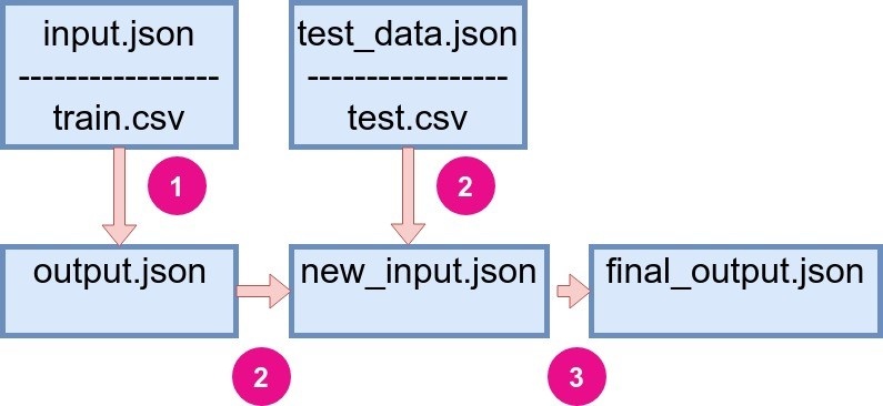
Figure 1: Recall on how StatwolfML flow is organized. |
The input.json file has the structure:
{
	“acquire”: {...},
	“preprocessing”: [...],
    “models”: [..]
}
In this section, we will work on the pre-processing aspect. It’s very simple with StatwolfML, since it has a very intuitive syntax and most of the function names are the same as in Panda’s and Sklearn Python libraries.
Let’s start with NaNs
From the explorative analysis, we know that columns “Age,” “Cabin,” and “Embarked,” contain null values. We won’t be using “Cabin” in our analysis due to the very large number of null values in it. Hence, we can just leave it as it is.
Note that “Embarked” is a categorical variable, while “Age” is the continuous one.
There are different strategies to fill the NaN values in the column. The simplest one is to just remove the lines containing NaNs. Another way is to impute these values. In StatwolfML, there are several ways to do that:
- impute_mean;
- impute_most_frequent;
- impute_median.
As it has been shown in the exploration part, the “Embarked” variable has three values: S, Q, and C, with S being most frequent. We can impute the NaN values for these columns as follows:
{
	“function”: “fillna”,
	“column”: “Embarked”,
	“value”: “S”
}
So, we have to specify function, name of the column, and value to be inserted in place of null. We could also use impute_most_frequent:
{
	“function”: “impute_most_frequent”,
	“column”: “Embarked”
}
For the “Age” column, we use the impute mean method since this is a continuous variable:
{
	“function”: “impute_mean”,
	“column”: “Age”
}
Note, that the mean value will be computed and for the unseen (test) dataset, the .json file will contain the following structure:
{
	“function”: “fillna”,
	“column”: “Age”,
	“value”: 29.699
}
This is to ensure that we have consistency between train and test datasets.
Feature Engineering
Transform continuous variables into categorical variables
We want to categorize the Fare column into four different groups:
| Range | Category |
|---|---|
| Fare 7.91 | 0 |
| 7.91 Fare 14.454 | 1 |
| 14.454 < Fare 31 | 2 |
| 31 < Fare | 3 |
These divisions are based on quantile discretization. We can do this by calling the encode_range function:
{
	“function” : “encode_range”,
	“columns”: [“Fare”],
	“range”: “x.Fare <= 7.91”,
	“value”: 0
}
We do the same for the rest of intervals.
In a similar manner, we transform the “Age” column to the categorical:
| Range | Category |
|---|---|
| Age 16 | 0 |
| 16 < Age 32 | 1 |
| 32 < Age 48 | 2 |
| 48 < Age 64 | 3 |
| 64 < Age | 4 |
For the “Sex” column, we use a different type of encoding, which is basically a mapping of non-numerical categorical values into numerical values:
{“Male”, “Female”} {0,1}
We just need to add the following code into the pre-process section:
{
    "function": "label_encoder",
    "columns": ["Sex"]
  }
Create a new column
StatwolfML permits us to perform simple feature engineering. In particular, one can create new columns combining the existing ones. Let’s see how it works.
First, we create a “Family” column, which is the combination of “Parch” and “SibSp.” Recall that these two columns describe family relations. “Parch,” is the parent-child columns and “SibSp,” is the sibling and spouse column. We sum them up in order to have one feature that describes familial relations:
{
	“function”: “create_column”,
	“new_col”: “Family”,
	“value”: “x[‘Parch’]+x[‘SibSp’]”
}
Hence, we added two columns that describe family members to one. Another column we want to add, is the combination of “Age” and “Pclass”:
{
	“function”: “create_column”,
	“new_col”: “age_class”,
	“value”: “x[‘Age’]*x[‘Pclass’]”
}
Basically, the user has to specify the name of the new column (“new col”) and add the operations (“value”).
Finalizing pre-process
The final two steps we need to do for the Titanic problem, is to encode the new column, “Family,” in a similar manner as we did for “Age” and “Fare”; then, we must remove the columns we do not need for the next steps.
So, for “Family,” we want to set the value at 1 if a passenger has a family member on board and 0 for all other cases:
{
	“function”:  “encode_range”,
	“columns”: [“Family”],
	“range”: “x.Family > 0”,
	“value”: 1
}
And, finally, let’s drop the columns that we no longer need:
{
    "function": "drop_columns",
    "columns": ["Name", "Ticket", "Embarked", "Cabin", "SibSp", "Parch", "Sex"]
  }
So, now what?
In the pre-processing part, we performed the following steps:
- Removed NaN values from the dataset using impute and fillna functions;
- Transformed continuous variables into categorical variables using the label_encoder function;
- Created new columns for further analysis;
- Dropped unnecessary columns from the dataset.
As you have seen, defining the pre-processing operations and flow in StatwolfML is both very easy and very flexible, too.
The main benefit is that, once you’ve done it, it can be applied to new data without worrying about missing steps, or making some errors (...as you know, that’s veeeery common :).
In the next blog post, we will see how to apply classification models inside StatwolfML and perform post-processing.