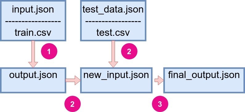
Just to help you recall the structure of the flow in StatwolfML, it consists of input.json and test_data.json files for both train and test functions, respectfully. The structure is depicted on Figure 1.
 |
|
Figure 1: Flow structure of StatwolfML. |
input.json file consist of following sections:
- acquire;
- preprocess;
- models;
- models_block;
- save.
And test_data.json:
- acquire;
- save.
How to define our machine learning data flow
Modelling
The input.json file we used for the preprocessing has the following structure:
{
	“acquire”: {...},
	“preprocessing”: [...],
    “models”: [..],
    “models_block”: [...]
}
We have already seen how to add the pre-process functions to the flow, and now we are focusing on the models section. Here, a user can list various models from the package. The general structure is given by:
“models”: [{
	“name”: “...”,
	“target_name”: “...”,
	“feature_names”: “...”
},{
	“name”: “...”,
	“target_name”: “...”,
	“feature_names” : “...”,
	“options” : {...}
}]
The parameters for each model are the following:
- name: a name of the model to use, defined in the package;
- target_name: name of the target columns for supervised models;
- feature_names: a list of feature names; all of the columns, excluding the target, will be taken if nothing is specified;
- label: a unique name for the model defined by user for the future references. If not specified, the name is used;
- options: options of the model; default is used if not specified.
models_block allows a user to use a list of models on the same set of features and target. The structure of it is the following:
“models_block”: [{
	“feature_names”: [...],
	“target_name”: ...,
	“accuracy_metrics”: [...],
	“models”: [...]
}]
Hence we can list various models in one block. A user can also define a list of evaluation metrics.
For the Titanic dataset, we will consider three different models: Logistic Regression, Support Vector Machine Classifier (SVC), and Decision Tree Classifier.
models_block": [{
    "target_name": "Survived",
    "accuracy_metrics": ["f1_score"],
    "models": [{
        "name": "logistic_regression",
        "label": "Logistic Regression"
        },
    {
        "name": "svc",
        "label": "SVC"
        },
    {
        "name": "decision_tree_classifier",
        "label": "Decision Tree Classifier"
        }]
    }]
Since we dropped unnecessary columns earlier in the pre-process section, we do not need specify the feature names - we will use the entire dataset.
Testing
The test_data.json has the following structure:
{
" acquire " : {
" source " : " filesystem" ,
" type " : " csv " ,
" dataset_name " : " titanic " ,
" address " : " example / titanic / test . csv " ,
" index_col " : 0
},

" save " : [ ]
}
There are three main parts:
- acquire: where we specify how the test dataset is downloaded;
- save: user can specify everything that needs to be set in the output. Basically, this is the same save-section as in the input flow. However, since the models were trained and applied, one can see the graphic outcome, save the results in file, etc.
Evaluate algorithms
Let us briefly explain the recall and precision metrics, and why they are important. Imagine as if we have a classification problem; we train a classifier on a dataset and then test it on unseen data.
| Category | Label | Prediction |
|---|---|---|
| True Positive | 1 | 1 |
| False Positive | 0 | 1 |
| False Negative | 1 | 0 |
| True Negative | 1 | 1 |
- True positive (TP) and true negative (TN) are those values which were correctly predicted.
- False positive (FP) and false negative (FN) are the values incorrectly predicted.
There are three different metrics available in order to estimate your classifier:
Accuracy
Accuracy measures how many samples that the algorithm correctly identifies.
In the Titanic user-case, the accuracy relates to the number of survived and non-survived values, which were predicted correctly and divided by the total number of samples.
Precision
Precision measures how many samples among those predicted as positive (TP+FP) are correct.
In our Titanic use-case, precision will tell you how many survivors are correctly identify by our model, over the total predicted survivors.
Recall
Recall measures how many samples that were classified as positve (TP+FN), are actually positive.
In the Titanic case, recall would identify how many survivors were identified correctly over the total number of survivors.
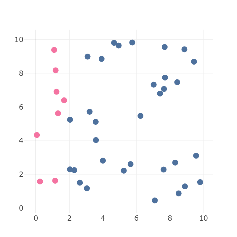
Why do we need to define three different metrics when we could just rely on precision? Well, imagine as if we dealt with skewed-data, when the number of negative values is much higher than the number of positive ones:
 |
|
Figure 2: Example of unbalanced dataset with two different values of labels. |
On Figure 2 we have:
- TN = 32,
- TP = 8,
- total = 40.
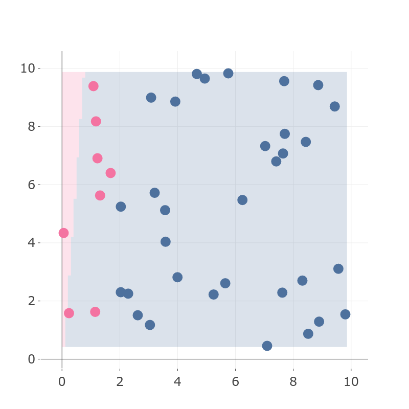
If the classifier predicts most of the samples to be blue, it will have good accuracy:
 |
|
Figure 3: Resulting classifier with high accuracy, where most of pink points are predicted as blue. |
On Figure 3, we see an example of a classifier. Let’s compute all of the components for the metrics:
- TP = 1,
- FP = 0,
- TN = 32,
- FN = 7.
And the metrics are:
- = 0.825,
- = 0.125.
Accuracy gets a high value, while precision is low. This means that we must take into account that possibility that only accuracy might be misleading when talking about the algorithm performance.
That is why precision and recall are more balanced metrics. A good algorithm has both high recall and high precision.
The metric that combines the two is called F1 score and it is given by:
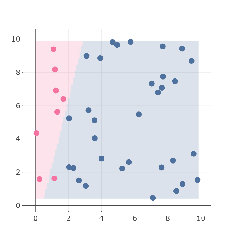
Going back to our example, a good classifier will give something like this:
 |
|
Figure 4: Example of a good classifier with high precision and high recall. |
Let us use this metric for the Titanic problem:
“accuracy_metrics”: [“f1_score”]Save our results
In a save section, we add the following:
" save " : [ {
" path " : " temp / titanic_final . csv " ,
" format " : " csv " ,
" outcome " : " filesystem "
} ,... ]
This declaration basically saves the dataset table with additional columns, the names of which are the model labels and the predicted values. And the last thing we want to put in the save section, are the plots:
" save " : [ ... ,
{
" outcome " : " filesystem " ,
" format " : " json " ,
" path " : " temp / log_reg . json " ,
" transform " : " plotly " ,
" figure " : [ {
" chartType " : " histogram " ,
" model " : " Logistic Regression "
}]
},
{
" outcome " : " filesystem " ,
" format " : " json " ,
" path " : " temp / dtc . json " ,
" transform " : " plotly " ,
" figure " : [ {
" chartType " : " histogram " ,
" model " : " Decision Tree Classifier "
}]
},
{
" outcome " : " filesystem " ,
" format " : " json " ,
" path " : " temp / svc . json " ,
" transform " : " plotly " ,
" figure " : [ {
" chartType " : " histogram " ,
" model " : " SVC "
}]
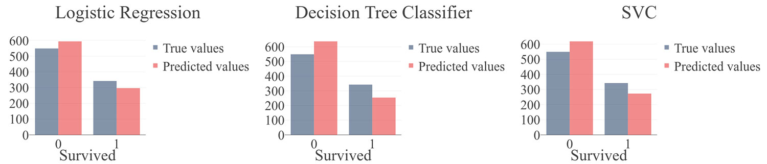
}]In the output file, we can find the accuracy score for each model in order to compare the performance of each algorithm. The results have shown that the SVC model has the highest F1 score (≈ 0.76, see the Figure 5).
 |
|
Figure 5: The results of three binary classifiers: (a) Logistic Regression, f1 ≈ 0.71, (b) Decision Tree Classifier, f1 ≈ 0.74 and (c) Support Vector Machine Classifier f1 ≈ 0.76. |
Let’s wrap everything up
We just concluded our first journey in StatwolfML, and we’ve seen:
- How to explore, visualise, and clean your dataset.
- How to define pre-processing, features engineering, and dataset preparation flows.
- How to set up your machine learning dataflow, and test and compare the results easily.
We tried to give you an overview on just how important it is for a data scientist to have a tool with:
- End-to-end machine learning capabilities (i.e. from data discovery, to deployment).
- Easy setup and maintenance (i.e. declarative syntax).
- Enough flexibility to tune and optimize results (i.e. data flows customisation).
We hope you enjoyed this introductory series of posts about StatwolfML, and we also hope to see you on the next series regarding Time Series analysis and forecast!